Ds
Data Structure#
Table of Contents
- Data Structure
- Introduction
- Array
- Linked List
- Stack
- Queue
- Hash
- Tree
- Desc
- Terminologies
- Why
- Application
- Hand Shaking Lemma
- Binary Tree
- Views
- Full Binary Tree
- Complete Binary Tree
- Perfect Binary Tree
- Degenerated / Pathological Tree
- Skew (Binary) Tree
- Left Skew (Binary) Tree
- Right Skew (Binary) Tree
- Binary Search Tree (BST)
- Self Balancing Binary Tree
- AVL Tree
- B-Tree
- Red-Black Tree
- B+ Tree
- K-ary Tree
- M-way Search Tree
- Heap
- Binary Heap
- Min Heap
- Max Heap
- Trie
- Graph
- References
- TODO
Introduction#
- Data structure (is a way) or (are the special format/structures in computer memory) to store & organize the data.
- To suit a specific purpose.
- So, that we can perform some operations on them like search, add, delete, insert
Data Structure Vs Data Type#
Data Type#
- It is class of objects sharing certain properties.
- It is a premitive element of a particular language like C, C++, Java, Python, Go
- Have predefined characteristics according to the language
- Contains data/information without any semantic
- Can't be reduced anymore
- e.g. integer, float, character, string, boolean
Data Structure#
- It is an abstract description of organization of data & operations on them
- It uses data types
- Can be decomposed to smaller
- DS are data type as well, but not a premitive type
Abstract Data Type (ADT)#
- Its visualization, thought, logical description, or a picture of a new data type which we are going to create
- while DS is a real & concrete thing, we can directly use them
DS is a super set and Data type is sub set or building block for DS
Types#
Linear Data Structure#
Traverses the data elements sequentially.
Only one data element can directly be reached.
- Array
- Linked List
- Singly Linked List
- Circular Linked List
- Doubly Linked List
- Stack
- Queue
- Hash
- Matrix
Non Linear Data Structure#
Every data item is attached to several other data items with a relationships.
The data items are not arranged in a sequential structure.
- Tree
- Binary Tree
- Full Binary Tree
- Complete Binary Tree
- Perfect Binary Tree
- Binary Search Tree - BST
- Degenerated / Pathological Tree
- Skew Binary Tree
- Left Skew Tree
- Right Skew Tree
- Binary Search Tree - BST
- Self Balancing / Balanced / Height Balanced BST
- AVL Tree
- B-tree
- Red-Black Tree
- B+ tree
- Splay Tree
- Treap
- Self Balancing / Balanced / Height Balanced BST
- K-ary Tree
- Heap
- Binary Heap
- Bionomial Heap
- Fibbonacci Heap
- Leftist Heap
- Skew Heap
- Trie
- Misc
- Indexing with Trees
- Segment Tree
- Fenwick Tree
- Binary Indexed Tree (BIT)
- Binomial Queues
- Open Hash Tables (Closed Addressing)
- Closed Hash Tables (Open Addressing)
- Closed Hash Tables, using buckets
- Binary Tree
- Graph
- Undirected Graph
- Directed Graph (Digraph)
- Directed Acyclic Graph (DAG)
- Directed Cyclic Graph [having cycle(s)] (DCG)
- Weighted
- Weighted Undirected Graph
- Weighted Directed Graph (WITHOUT negative weights)
- Weighted DAG
- Weighted DCG
- Weighted Directed Graph (WITH negative weights)
- Weighted DAG
- Weighted DCG
- WITH Negative Weight Cycle
- WITHOUT Negative Weight Cycle
- Misc
- Finite Graph
- Infinite Graph
- Trivial Graph
- Simple Graph
- Multi Graph
- Null Graph (Empty Graph)
- Complete Graph
- Pseudo Graph
- Regular Graph
- Bipartite Graph
- Labelled Graph
- Connected & Disconnected Graph
- Cyclic Graph
- Vertex Labelled Graph
- Subgraph
- Rooted Graph
- Mixed Graph
- Path Graph
- Planar Graph
- Cycle Graph
- Petersen Graph
- Perfect Graph
- Cograph
- Chordal Graph
- Misc
- Disjoint-set Data Structures
- Suffix Arrays
Language Specific#
- Python
- list
- tuple
- set
- dict
- built-in dict
- collections.OrderedDict
- remember insertion order of keys
- collections.defaultdict
- return default values for missing keys
- collections.ChainMap
- search multiple dicts as a single mapping
- types.MappingProxyType
- A wrapper for making read-only dictionaries
- Java
- C#
- Go
Array#
Linked List#
Doubly Linked List#
Circular Linked List#
Stack#
LIFO
Queue#
FIFO
Simple Queue#
Circular Queue#
Dequeue#
(aka Doubly eneded queue)
Priority Queue#
Desc#
Application#
- job scheduling
- event-driven simulation
Properties#
Operations#
- INSERT
- MAXIMUM
- EXTRACT-MAX
- REPLACE
Implementation#
- Array/Set/List(LinkedList)
- Binary Heap
- Fibbonacci Heap
Hash#
Desc#
- Linear data structure (ADT) to make lookup fast
- uses a hashing functions, a slot list and, a data list
- time complexity (lookup):
- best: O(1)
- worst: O(n)
Terminologies#
- hash function
- folding method
- mid-squared method
- perfect hash functions
- slot/bucket
- load factor
- collision
- resolution techniques (rehashing)
- open addressing
- linear probing
- quadratic probing
- disadvantages
- clustered data
- chaining
- open addressing
- resolution techniques (rehashing)
Why#
- to optimize the look-up speed after binary search and other varients
Dictionary#
- a general concept/data structure that maps keys to values
- many ways to implement dictionary
- hashtable; O(1) - O(N)
- red-black tree; always O(longN)
Hash Table#
- synchronized
- thread safe
- can be shared with many threads
- doesn't allows any null key or values
Hash Map#
- non synchronized
- non-thread safe
- can't be shared between many threads without proper synchronization code
- allows one null key and multiple null values
- preferred over hash-table
Tree#
Desc#
- Are hierchical data structure
- made up of nodes or vertices and edges without having any cycle
- The tree with no nodes is called the null or empty tree
Terminologies#
- Root: The top node in a tree
- Child: A node directly connected to another node when moving away from the Root
- Parent: The converse notion of a child
- Siblings: A group of nodes with the same parent
- Descendant: A node reachable by repeated proceeding from parent to child
- Ancestor: A node reachable by repeated proceeding from child to parent
- Leaf: (less commonly called External node) A node with no children
- Branch: Internal node, A node with at least one child
- Degree: The number of subtrees of a node
- Edge: The connection between one node and another
- Path: A sequence of nodes and edges connecting a node with a descendant
- Depth of node: The depth of a node is the number of edges from the tree's root node to the node
- Level of node: All nodes of depth d are at level d
- Height of node: The height of a node is the number of edges on the longest path between that node and a leaf
- Depth & Level of root node is zero (some may say 1 as well - no problem)
- Depth & Level are measured from top (root) to bottom (leaf)
- Height is measured from bottom (leaf) to top (root)
- Height of the leaf in last level is zero
- Depth of tree: The number of edges between root & deepest leaf + 1
- Level of tree: The number of levels in the tree (i.e. number of edges between root & deepest leaf + 1; i.e. same as Depth of tree)
- Height of tree: The height of a tree is the height of its root node using longest path
- Forest: A forest is a set of n \ge 0 disjoint trees
Why#
- need to store in hierchical way, e.g. computer filesystem
- provides quicker insertion/deletion than array but slower than unordered linked list
- No upper limit on number of nodes (like linkedlist & unlike array)
Application#
- Easy to search (using traversal)
- Router Algorithm
- decision making
Hand Shaking Lemma#
In an undirected graph, Number of vertex of odd degree are always even
e.g. Vertex of odd degree = Vertex connected to 3 edges.
Binary Tree#
Desc#
- tree whose each node have at most 2 children
- children typically known as left and right child
Representation#
- a node consist of data, pointer to left child, pointer to right child
Array Representation#
- Root at index 0
- Left child at index 2 \times i
- Right child at index 2 \times i + 1
- Parent at index i / 2
Note:
- The array should be filled with nil value for non-existing child nodes
- i.e. if traverse level-by-level, then if there are any missing nodes, then the index of those nodes should be filled with nil values
Properties#
- Level(Root) = 0
- Height of tree with only root node = 0
- Maximum number of nodes possible at level i is 2^{i}
- Maximum number of nodes possible in a binary tree of height h is 2^{h+1}-1
- no. of Levels in a Tree = Height of the Tree + 1
- Minimum Possible Height of a tree having N nodes: h = \lfloor \log_2{(N+1)} \rfloor
- A binary tree with L leaves is of at least height h = \lceil \log_2{L} \rceil
- Number of leaves = Number of internal nodes having 2 children + 1
Operations#
Depth First Traversal#
- Types:
- In Order: left, root, right
- Pre Order: root, left, right
- Post Order: left, right, root
- Ways:
- Standard (Recursive)
- Desc:
- Approach: Recursive
- DS Used:
- Using Stack (Iterative, Which is same as Recursive one)
- Desc:
- Apprach: Iterative
- DS Used: Stack
- Without Recursion, Without Stack: Morris Traversal: Based on Threaded Binary Tree
- Desc:
- Apprach:
- DS Used:
- Standard (Recursive)
- Time Complexity: O(n)
- Auxilary Space:
- Avg: O(h) due to Recursive call stack; where h is max height of the tree
- Worst: When tree is skewed tree, i.e. h at last level = O(\log_2{n})
- Dis-Advantage:
- Recursive solution
- Traversal starts from Leaf, unlike BFS.
Breadth First Traversal (Level Order Traversal)#
- Way:
- Using Level By Level Looping:
- Desc:
- Find out total level of the tree : Traverse each sub-tree + Compare level of left & right
- Loop from first level to last
- For each level print all the nodes:
- If root is empty, return; If level reached 1, print the data
- Make Recursive call for each child by decreasing level by 1
- Approach: Recursive
- DS Used: None
- Desc:
- Using Queue
- Desc:
- If given node is not none, visit & print given node,
- Then enqueue left & right child in the queue (if they are not none).
- Dequeue one node from the queue & make recursive call for that node.
- Approach: Recursive
- DS Used: Queue
- Desc:
- Using Level By Level Looping:
- Time Complexity: \theta{(n)}
- Auxilary Space:
- Avg: O(w), where w is max width of the tree
- Worst: When tree is Perfect tree, i.e. w at last level = O(\lceil {n/2} \rceil)
- Advantage:
- Non recursive solution
- Traversal starts from root, unlike DFS. So, better if our finding is closer to root.
Vertical Order Traversal#
When nodes are traversed in vertical lines.
1 2 3 4 5 6 7 8 9 10 11 12 13 14 15 16 | |
TODO
Views#
Top View of a binary tree#
Top view of a binary tree is the set of nodes visible when the tree is viewed from the top.
Imagine a real X-mas tree, and view it from sky.
Note: Order of nodes doesn't matter.
1 2 3 4 5 6 7 8 9 10 11 12 13 14 15 16 17 18 19 | |
Bottom View of a binary tree#
Bottom view of a binary tree is the set of nodes visible when the tree is viewed from the bottom.
Horizontal distance of node: The distance of a node from root, when measured horizontally (say in x-axis). And suppose root node lies on y-axis (i.e. x=0).
So, another definition of bottom view:
Set of bottommost nodes at their horizontal distance, i.e. For each horizontal distance unit, pick the bottom most node.
Note: If there are two bottom most nodes at same horizontal distance, then pick the last/right one.
1 2 3 4 5 6 7 8 9 10 11 12 13 14 15 16 17 18 19 20 | |
Left View of a binary tree#
Left view of a binary tree is the set of nodes visible when the tree is viewed from the left-side.
Right View of a binary tree#
Right view of a binary tree is the set of nodes visible when the tree is viewed from the right-side.
Full Binary Tree#
Every node at a particular level has 0 or 2 children
Complete Binary Tree#
All level are completely filled, except possibly last level and last level has all keys as left as possible.
Practical e.g.: Binary Heap
1 2 3 4 5 6 7 8 9 10 11 12 13 14 15 | |
Properties#
- height of a complete binary tree (having N nodes) = \log_2{N}
Perfect Binary Tree#
All internal nodes have 2 children and all leaves are at same level.
Degenerated / Pathological Tree#
Every internal node has one child. Performance-wise same as linked list.
Skew (Binary) Tree#
A tree with every node having one child only
Left Skew (Binary) Tree#
A tree with every node having one Left child only
Right Skew (Binary) Tree#
A tree with every node having one Right child only
Binary Search Tree (BST)#
Desc#
Operations#
- SEARCH, MINIMUM, MAXIMUM, PREDECESSOR, SUCCESSOR, INSERT, DELETE
Self Balancing Binary Tree#
(aka Balanced / Height Balanced BST)
To over come the downside of the skewed BST, (when its search performance degrades to linear time), various self-balancing BST were proposed around 1962 - 1973.
- AVL Tree [1962]
- B-tree [1970]
- Red-Black Tree [1972]
- B+ tree [1972-73]
- Splay Tree
- Treap
AVL Tree#
First self-balancing BST to overcome the limitations of BST when its skewed.
| Invented | By |
|---|---|
| 1962 | Georgy Adelson-Velsky & Evgenii Landis |
Specification#
- While creating/updating a BST, if the heights of the two child subtree of a node differs by more than 1, then rebalance that node
- Rebalancing is done by performing single or double-step rotation
- Note: Try to rebalance the BST as soon as possible.
Rotation#
LL (left-left) Rotation#
1 2 3 4 5 | |
Here, the balance factor of the:
- node 3
- = height of left subtree - height of right tree
- = 0 - 0
- = 0
- node 4
- = height of left subtree - height of right tree
- = 1 - 0
- = 1
- node 5
- = height of left subtree - height of right tree
- = 2 - 0
- = 2
The balance factor of 5 is not in -1,0,1 (i.e. imbalanced by more than 1). Thus node 5 is imbalanced due to recent addition of node 3, to which we can reach by following "Left-->Left" i.e. LL.
Thus node 5 is said to be LL imbalanced.
To fix that, rotate the tree around 5 such that, 4 becomes parent of 3 & 5.
(Assume putting a nail under node 5 and pulling 5 1-step towards right)
i.e.
1 2 3 | |
Thus, it is called LL-rotation.
RR (right-right) Rotation#
1 2 3 4 5 | |
Similarly this is called RR imbalance.
If we rotate the tree around node 5, such that node 7 become the parent of the 5 & 9. i.e.
1 2 3 | |
Then, this is called RR rotation.
LR (left-right) Rotation#
1 2 3 4 5 | |
Here, the balance factor of the:
- node 6
- = height of left subtree - height of right tree
- = 0 - 0
- = 0
- node 5
- = height of left subtree - height of right tree
- = 0 - 1
- = -1
- node 7
- = height of left subtree - height of right tree
- = 2 - 0
- = 2
The balance factor of 7 is not in -1,0,1 (i.e. imbalanced by more than 1). Thus node 7 is imbalanced due to recent addition of node 6, to which we can reach by following "Left-->Right" i.e. LR.
Thus node 7 is said to be LR imbalanced.
To fix that, follow a 2-step rotation:
-
swap the node 5 & 6 (doing so, we achieved LL imbalanced state; Note: we changed the side as well)
1
2
3
4
5
7 / 6 / 5 -
now follow the LL rotation (i.e. rotate the tree around 7 such that, 6 becomes parent of 5 & 7. i.e.
1
2
3
    6
   / \
  5   7
RL (right-left) Rotation#
1 2 3 4 5 | |
Similarly this is called RL imbalance.
If we:
-
swap the node 7 and 6
1
2
3
4
5
5 \ 6 \ 7 -
rotate the tree around node 5, such that node 6 become the parent of the 5 & 7. i.e.
1
2
3
  6
 / \
5   7
Then, this is called RL rotation.
The shorthand for this 2-step rotation could be:
Replace Parent (node 5) with node L (node 6) and make the Parent (node 5) L child of node 6.
Exercise#
Q1.
1 2 3 4 5 | |
A.
1 2 3 4 5 | |
Q2.
1 2 3 4 5 | |
A.
1 2 3 4 5 | |
Q3.
1 2 3 4 5 6 7 8 9 | |
A.
Addition of 4 causes LLRL (no just call it LL) imbalance of node 7.
Now, just focus on node 3, 6, and 7 (as we do in LL rotation).
1 2 3 4 5 6 7 | |
Complexity#
| Of | Avg | Worst |
|---|---|---|
| Space | \Theta(n) | O(n) |
| Search | \Theta(log_2{n}) | O(log_2{n}) |
| Insert | \Theta(log_2{n}) | O(log_2{n}) |
| Delete | \Theta(log_2{n}) | O(log_2{n}) |
B-Tree#
(aka Balanced/Bayer/Boeing/Broad/Bushy Tree)
First self-balancing m-way Search Tree (ST) to overcome the limitations of m-way ST when its skewed.
| Invented | By |
|---|---|
| 1970 | Rudolf Bayer & Edward M. McCreight while working at Boeing Research Labs |
Idea: While creating/updating a BST, if the heights of the two child subtree of a node differs by more than 1, then rebalance that node.
I see it as:
- generalization of the AVL tree
- self balanced version of m-way search tree
Application#
- Indexing in Databases
- Filesystem
Specification#
- defined by order of the tree
- order = number of children
- size of key = order - 1
- nodes should be half full
- root can have less than half order
- keys are in sorted order for sequential traversal
- a B-tree of height h with all its nodes completely filled has n = m^{h+1}–1 entries
- minimum height of a b-tree: TODO
- maximum height of a b-tree: TODO
Complexity#
| Of | Avg | Worst |
|---|---|---|
| Space | \Theta(n) | O(n) |
| Search | \Theta(log_2{n}) | O(log_2{n}) |
| Insert | \Theta(log_2{n}) | O(log_2{n}) |
| Delete | \Theta(log_2{n}) | O(log_2{n}) |
Red-Black Tree#
B+ Tree#
K-ary Tree#
M-way Search Tree#
Heap#
- Heap are nothing but a speacial form of tree
- The special condition is:
- the value of a node MUST be \ge (or \le ) value of its children (heap property)
- notice its different than BST
- the value of a node MUST be \ge (or \le ) value of its children (heap property)
- Another good to have condition is (not mandatory, but good for performance)
- all the levels should be fullfilled, except the possible last
- i.e. all the leaves should be in the level l or l-1 (suppose l is height of the tree/root, for l \gt 0)
- i.e. the heap should be a complete binary tree
- reason:
- it will guarantee O(log_{2} N) to build operation
- it will guarantee O(log_{2} N) to insert operation
- because both depends on the height of the heap
- and height = log_{2} N, where N is size of the heap
Binary Heap#
A heap with atmost 2 children
Applications#
- Heap Sort: Heap Sort uses Binary Heap to sort an array in O(nLogn) time.
- Priority Queue: Priority queues can be efficiently implemented using Binary Heap because it supports insert(), delete() and extractmax(), decreaseKey() operations in O(logn) time. Binomoial Heap and Fibonacci Heap are variations of Binary Heap. These variations perform union also efficiently.
- Graph Algorithms: The priority queues are especially used in Graph Algorithms like Dijkstra’s Shortest Path and Prim’s Minimum Spanning Tree.
- Many problems likes
- K’th Largest Element in an array.
- Sort an almost sorted array/
- Merge K Sorted Arrays.
Min Heap#
A binary heap in which the value of a node MUST be \le value of its children
Operations#
- Insertion
- Top/Min
- Delete-Top / Extract-Min (Get & Delete) Top
- Replace
Max Heap#
A binary heap in which the value of a node MUST be \ge value of its children
Operations#
- Insertion
- Top/Max
- Delete-Top / Extract-Max (Get & Delete) Top
- Replace
Implementations#
| Implementation | Insert | Delete-Max | Extract-Min |
|---|---|---|---|
| Unordered Array | 1 | n | n |
| Unordered List | 1 | n | n |
| Ordered Array | n | 1 | 1 |
| Ordered List | n | 1 | 1 |
| Binary Search Tree | log n | log n | log n |
| Balanced Binary Search Tree | log n | log n | log n |
| Binary Heaps | log n | log n | 1 |
Operations#
Trie#
Graph#
G = (V, E)
Desc#
- a data structure describing pairwise relations between objects
- made up of nodes/vertices and edges; with or without having any cycle
- sometimes called undirected graph for distinguishing from a directed graph, or simple graph for distinguishing from a multigraph
Terminologies#
- Vertex (Node/Point): fundamental unit of the graph;
- Edge (Link/Line/Arc): The connection between one vertex and another
- Degree (of a Vertex):
𝛿(v)in a graph is the number of edges incident to it - In Degree:
𝛿 -(v)number of incoming edges - Out Degree:
𝛿 +(v)number of outgoing edges - Adjacent Vertex: vertices directly connected to the given vertex
- Adjacency Matrix:
Size: VxVa matrix denoting (ordered/unordered) relations/edge between all the vertices - Adjacency List: a map of size
Vof list/linkedlist denoting vertices connected to a particular vertex - Isolated Vertex: is a vertex with degree zero
- Leaf Vertex (Pendant Vertex): is a vertex with degree one
- Source vertex: is a vertex with indegree zero
- Sink vertex: is a vertex with outdegree zero
- Simplicial vertex: is one whose neighbors form a clique: every two neighbors are adjacent
- Universal vertex: is a vertex that is adjacent to every other vertex in the graph
- Cut vertex: is a vertex the removal of which would disconnect the remaining graph
- Tree: A graph with no cycle; aka Acyclic Connected Graph
- Forest: is a disjoint set (non-overlapping elements in each set) iof trees
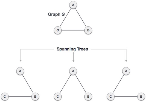
-
Spanning Tree: A subset of a graph, such that it covers all the vertices of the graph but with minimal edges.
- Thus, it does NOT have any cycle
- It is NOT disconncted
- Can say, every connected & undirected graphs have atleast 1 spanning tree
-
Connected components: A connected component or simply component of an undirected graph is a subgraph in which each pair of nodes is connected with each other via a path
- Strongly connected components (SCC): In a directed graph if every vertex is reachable from every other vertex
Why#
- need to store network of objects / relations between objects
- e.g.
- a map of cities
- social n/w
- to describe such complicated thing in less space
- e.g.
Application#
- transport networks
- computer networks
- database relationships
- relationships between electronic components
Representation#
Adjacency Matrix#
A matrix (2-d array) denoting if there is an edge (directed/undirected) between 2 vertices or not.
1
2
3
4
5
6
| |
- Size: V*V
- Advantages
- Some operations are efficient and easy
- Disadvantages
- More space
- could be wastage if the graph is sparse (not dense)
- More space
Adjacency List#
A array of list (or a map of list) denoting adjacent vetices of a particular vertex.
1 2 3 4 | |
- Size: E + V
- Advantages
- less space than adjacency matrix
- especially when the graph is not dense
- less space than adjacency matrix
- Disadvantages
- some operations are not efficient using adjacency list
- where lookup (whether there is an edge between 2 vertices or not) is required
- deleting a vertex
- deleting an edge
- some operations are not efficient using adjacency list
Adjacency Set#
TODO
Operations#
- Addition
- Add Node
- Add Edge
- Removal
- Remove Node
- Remove Edge
- Search
- Contains - check if the graph contains a given value
- HasEdge - check if there is an edge between 2 given vertices
- Traversal - traverse the graph & its nodes/edges in various fashion
Undirected Graph#
Directed Graph#
Directed Acyclic Graph (DAG)#
Directed Cyclic Graph (DCG)#
Weighted Graph#
Subgraph#
A graph whose edge & veritices are subset of the other graph.
Bipartite Graph#
A graph whose vertices could be divided/partitioned into 2 sets. Such that vertices of one set incidents an edge to verices on the other set.

Complete Graph#
A graph whose all the vertices are connected to each other. aka A graph whose all the edges are present.
1 | |
Sparse Graph#
A graph with relatively less edges.
1 | |
Dense Graph#
A graph with relatively less edges are missing.
References#
- https://gist.github.com/toransahu/bb1c9f1cd6490ff29c42fa229e827a2a
TODO#
- avl
- m-way tree
- b tree
- b+ tree
- red-black tree
- trie